Array Formulas
Many of the formulas described here are Array Formulas, which are a special type of formula
in Excel. If you are not familiar with Array Formulas, click here.
Array To Column
Sometimes it is useful to convert an MxN array into a single column of data, for example for charting (a data series must be a single row or column). Clickhere for more details.
Averaging Values In A Range
You can use Excel's built in =AVERAGE function to average a range of values. By using it
with other functions, you can extend its functionality.
For the formulas given below, assume that our data is in the range A1:A60.
Averaging Values Between Two Numbers
Use the array formula
=AVERAGE(IF((A1:A60>=Low)*(A1:A60<=High),A1:A60))
Where Low and High are the values between which you want to average.
Averaging The Highest N Numbers In A Range
To average the N largest numbers in a range, use the array formula
=AVERAGE(LARGE(A1:A60,ROW(INDIRECT("1:10"))))
Change "1:10" to "1:N" where N is the number of values to average.
Averaging The Lowest N Numbers In A Range
To average the N smallest numbers in a range, use the array formula
=AVERAGE(SMALL(A1:A60,ROW(INDIRECT("1:10"))))
Change "1:10" to "1:N" where N is the number of values to average.
In all of the formulas above, you can use =SUMinstead of =AVERAGE to sum, rather
than average, the numbers.
Counting Values Between Two Numbers
If you need to count the values in a range that are between two numbers, for example between
5 and 10, use the following array formula:
=SUM((A1:A10>=5)*(A1:A10<=10))
To sum the same numbers, use the following array formula:
=SUM((A1:A10>=5)*(A1:A10<=10)*A1:A10)
Counting Characters In A String
The following formula will count the number of "B"s, both upper and lower case, in the string in B1.
=LEN(B1)-LEN(SUBSTITUTE(SUBSTITUTE(B1,"B",""),"b",""))
Date And Time Formulas
A variety of formulas useful when working with dates and times are described on
the DateTime page.
Other Date Related Procedures are described on the following pages.
Adding Months And Years
The DATEDIF Function
Date Intervals
Dates And Times
Date And Time Entry
Holidays
Julian Dates
Duplicate And Unique Values In A Range
The task of finding duplicate or unique values in a range of data requires some complicated
formulas. These procedures are described inDuplicates.
Dynamic Ranges
You can define a name to refer to a range whose size varies depending on its contents. For example, you may want a range name that refers only to the portion of a list of numbers that are not blank. such as only the first N non-blank cells in A2:A20. Define a name called MyRange, and set the Refers To property to:
=OFFSET(Sheet1!$A$2,0,0,COUNTA($A$2:$A$20),1)
Be sure to use absolute cell references in the formula. Also see then Named Ranges page for more information about dynamic ranges.
Finding The Used Part Of A Range
Suppose we've got a range of data calledDataRange2, defined as H7:I25, and that
cells H7:I17 actually contain values. The rest are blank. We can find various properties
of the range, as follows:
To find the range that contains data, use the following array formula:
=ADDRESS(ROW(DataRange2),COLUMN(DataRange2),4)&":"&
ADDRESS(MAX((DataRange2<>"")*ROW(DataRange2)),COLUMN(DataRange2)+
COLUMNS(DataRange2)-1,4)
This will return the range H7:I17. If you need the worksheet name in the returned range,
use the following array formula:
=ADDRESS(ROW(DataRange2),COLUMN(DataRange2),4,,"MySheet")&":"&
ADDRESS(MAX((DataRange2<>"")*ROW(DataRange2)),COLUMN(DataRange2)+
COLUMNS(DataRange2)-1,4)
This will return MySheet!H7:I17.
To find the number of rows that contain data, use the following array formula:
=(MAX((DataRange2<>"")*ROW(DataRange2)))-ROW(DataRange2)+1
This will return the number 11, indicating that the first 11 rows of DataRange2 contain data.
To find the last entry in the first column ofDataRange2, use the following array formula:
=INDIRECT(ADDRESS(MAX((DataRange2<>"")*ROW(DataRange2)),
COLUMN(DataRange2),4))
To find the last entry in the second column ofDataRange2, use the following array formula:
=INDIRECT(ADDRESS(MAX((DataRange2<>"")*ROW(DataRange2)),
COLUMN(DataRange2)+1,4))
First And Last Names
Suppose you've got a range of data consisting of people's first and last names.
There are several formulas that will break the names apart into first and last names
separately.
Suppose cell A2 contains the name "John A Smith".
To return the last name, use
=RIGHT(A2,LEN(A2)-FIND("*",SUBSTITUTE(A2," ","*",LEN(A2)-
LEN(SUBSTITUTE(A2," ","")))))
To return the first name, including the middle name (if present), use
=LEFT(A2,FIND("*",SUBSTITUTE(A2," ","*",LEN(A2)-
LEN(SUBSTITUTE(A2," ",""))))-1)
To return the first name, without the middle name (if present), use
=LEFT(B2,FIND(" ",B2,1))
We can extend these ideas to the following. Suppose A1 contains the
string "First Second Third Last".
Returning First Word In A String
=LEFT(A1,FIND(" ",A1,1))
This will return the word "First".
Returning Last Word In A String
=RIGHT(A1,LEN(A1)-MAX(ROW(INDIRECT("1:"&LEN(A1))) *(MID(A1,ROW(INDIRECT("1:"&LEN(A1))),1)=" ")))
This formula in as array formula.
(This formula comes from Laurent Longre). This will return the word "Last"
Returning All But First Word In A String
=RIGHT(A1,LEN(A1)-FIND(" ",A1,1))
This will return the words "Second Third Last"
Returning Any Word Or Words In A String
The following two array formulas come compliments of Laurent Longre. To return any single word from a single-spaced string of words, use the following array formula:
=MID(A10,SMALL(IF(MID(" "&A10,ROW(INDIRECT
("1:"&LEN(A10)+1)),1)=" ",ROW(INDIRECT("1:"&LEN(A10)+1))),
B10),SUM(SMALL(IF(MID(" "&A10&" ",ROW(INDIRECT
("1:"&LEN(A10)+2)),1)=" ",ROW(INDIRECT("1:"&LEN(A10)+2))),
B10+{0,1})*{-1,1})-1)
Where A10 is the cell containing the text, and B10 is the number of the word you want to get.
This formula can be extended to get any set of words in the string. To get the words from M for N words (e.g., the 5th word for 3, or the 5th, 6th, and 7th words), use the following array formula:
=MID(A10,SMALL(IF(MID(" "&A10,ROW(INDIRECT
("1:"&LEN(A10)+1)),1)=" ",ROW(INDIRECT("1:"&LEN(A10)+1))),
B10),SUM(SMALL(IF(MID(" "&A10&" ",ROW(INDIRECT
("1:"&LEN(A10)+2)),1)=" ",ROW(INDIRECT("1:"&LEN(A10)+2))),
B10+C10*{0,1})*{-1,1})-1)
Where A10 is the cell containg the text, B10 is the number of the word to get, and C10 is the number of words, starting at B10, to get.
Note that in the above array formulas, the {0,1}and {-1,1} are enclosed in array braces (curly brackets {} ) not parentheses.
Download a workbook illustrating these formulas.
Grades
A frequent question is how to assign a letter grade to a numeric value. This is simple. First create a define name called "Grades" which refers to the array:
={0,"F";60,"D";70,"C";80,"B";90,"A"}
Then, use VLOOKUP to convert the number to the grade:
=VLOOKUP(A1,Grades,2)
where A1 is the cell contains the numeric value. You can add entries to the Grades array for other grades like C- and C+. Just make sure the numeric values in the array are in increasing order.
High And Low Values
You can use Excel's Circular Reference tool to have a cell that contains the highest ever reached value. For example, suppose you have a worksheet used to track team scores. You can set up a cell that will contain the highest score ever reached, even if that score is deleted from the list. Suppose the score are in A1:A10. First, go to the Tools->Options dialog, click on the Calculation tab, and check the Interations check box. Then, enter the following formula in cell B1:
=MAX(A1:A10,B1)
Cell B1 will contian the highest value that has ever been present in A1:A10, even if that value is deleted from the range. Use the =MIN function to get the lowest ever value.
Another method to do this, without using circular references, is provided by Laurent Longre, and uses the CALL function to access the Excel4 macro function library. Click here for details.
Left Lookups
The easiest way do table lookups is with the=VLOOKUP function. However, =VLOOKUP requires
that the value returned be to the right of the value you're looking up. For example, if you're
looking up a value in column B, you cannot retrieve values in column A. If you need to
retrieve a value in a column to the left of the column containing the lookup value, use
either of the following formulas:
=INDIRECT(ADDRESS(ROW(Rng)+MATCH(C1,Rng,0)-1,COLUMN(Rng)-ColsToLeft)) Or
=INDIRECT(ADDRESS(ROW(Rng)+MATCH(C1,Rng,0)-1,COLUMN(A:A) ))
Where Rng is the range containing the lookup values, and ColsToLeft is the number of columns
to the left of Rng that the retrieval values are. In the second syntax, replace "A:A" with the
column containing the retrieval data. In both examples, C1 is the value you want to look up.
See the Lookups page for many more examples of lookup formulas.
Minimum And Maximum Values In A Range
Of course you can use the =MIN and =MAX functions to return the minimum and maximum
values of a range. Suppose we've got a range of numeric values called NumRange.
NumRange may contain duplicate values. The formulas below use the following example:

Address Of First Minimum In A Range
To return the address of the cell containing the first(or only) instance of the minimum of a list,
use the following array formula:
=ADDRESS(MIN(IF(NumRange=MIN(NumRange),ROW(NumRange))),COLUMN(NumRange),4)
This function returns B2, the address of the first '1' in the range.
Address Of The Last Minimum In A Range
To return the address of the cell containing the last(or only) instance of the minimum of a list,
use the following array formula:
=ADDRESS(MAX(IF(NumRange=MIN(NumRange),ROW(NumRange)*(NumRange<>""))),
COLUMN(NumRange),4)
This function returns B4, the address of the last '1' in the range.
Address Of First Maximum In A Range
To return the address of the cell containing the firstinstance of the maximum of a list,
use the following array formula:
=ADDRESS(MIN(IF(NumRange=MAX(NumRange),ROW(NumRange))),COLUMN(NumRange),4)
This function returns B1, the address of the first '5' in the range.
Address Of The Last Maximum In A Range
To return the address of the cell containing the lastinstance of the maximum of a list,
use the following array formula:
=ADDRESS(MAX(IF(NumRange=MAX(NumRange),ROW(NumRange)*(NumRange<>""))),
COLUMN(NumRange),4)
This function returns B5, the address of the last '5' in the range.
Download a workbook illustrating these formulas.
Most Common String In A Range
The following array formula will return the most frequently used entry in a range:
=INDEX(Rng,MATCH(MAX(COUNTIF(Rng,Rng)),COUNTIF(Rng,Rng),0))
Where Rng is the range containing the data.
Ranking Numbers
Often, it is useful to be able to return the N highest or lowest values from a range of data.
Suppose we have a range of numeric data calledRankRng. Create a range next to
RankRng (starting in the same row, with the same number of rows) called TopRng.
Also, create a named cell called TopN, and enter into it the number of values you want to
return (e.g., 5 for the top 5 values in RankRng). Enter the following formula in the first cell in
TopRng, and use Fill Down to fill out the range:
=IF(ROW()-ROW(TopRng)+1>TopN,"",LARGE(RankRng,ROW()-ROW(TopRng)+1))
To return the TopN smallest values of RankRng, use
=IF(ROW()-ROW(TopRng)+1>TopN,"",SMALL(RankRng,ROW()-ROW(TopRng)+1))
The list of numbers returned by these functions will automatically change as you change the
contents of RankRng or TopN.
Download a workbook illustrating these formulas.
See the Ranking page for much more information about ranking numbers in Excel.
Removing Blank Cells In A Range
The procedures for creating a new list consisting of only those entries in another list, excluding
blank cells, are described in NoBlanks.
Summing Every Nth Value
You can easily sum (or average) every Nth cell in a column range. For example, suppose you want to sum every 3rd cell.
Suppose your data is in A1:A20, and N = 3 is inD1. The following array formula will sum the values in A3, A6, A9, etc.
=SUM(IF(MOD(ROW($A$1:$A$20),$D$1)=0,$A$1:$A$20,0))
If you want to sum the values in A1, A4, A7, etc., use the following array formula:
=SUM(IF(MOD(ROW($A$1:$A$20)-1,$D$1)=0,$A$1:$A$20,0))
If your data ranges does not begin in row 1, the formulas are slightly more complicated. Suppose our data is in B3:B22, and N = 3 is in D1. To sum the values in rows 5, 8, 11, etc, use the followingarray formula:
=SUM(IF(MOD(ROW($B$3:$B$22)-ROW($B$3)+1,$D$1)=0,$B$3:B$22,0))
If you want to sum the values in rows 3, 6, 9, etc, use the following array formula:
=SUM(IF(MOD(ROW($B$3:$B$22)-ROW($B$3),$D$1)=0,$B$3:B$22,0))
Download a workbook illustrating these formulas.
Miscellaneous
Sheet Name
Suppose our active sheet is named "MySheet" in the file C:\Files\MyBook.Xls.
To return the full sheet name (including the file path) to a cell, use
=CELL("filename",A1)
Note that the argument to the =CELL function is the word "filename" in quotes, not your
actual filename.
This will return "C:\Files\[MyBook.xls]MySheet"
To return the sheet name, without the path, use
=MID(CELL("filename",A1),FIND("]",CELL("filename",A1))+1,
LEN(CELL("filename",A1))-FIND("]",CELL("filename",A1)))
This will return "MySheet"
File Name
Suppose our active sheet is named "MySheet" in the file C:\Files\MyBook.Xls.
To return the file name without the path, use
=MID(CELL("filename",A1),FIND("[",CELL("filename",A1))+1,FIND("]",
CELL("filename",A1))-FIND("[",CELL("filename",A1))-1)
This will return "MyBook.xls"
To return the file name with the path, use either
=LEFT(CELL("filename",A1),FIND("]",CELL("filename",A1)))Or
=SUBSTITUTE(SUBSTITUTE(LEFT(CELL("filename",A1),FIND("]",
CELL("filename",A1))),"[",""),"]","")
The first syntax will return "C:\Files\[MyBook.xls]"
The second syntax will return "C:\Files\MyBook.xls"
In all of the examples above, the A1 argument to the=CELL function forces Excel to get the sheet name from the sheet containing the formula. Without it, and Excel calculates the =CELL function when another sheet is active, the cell would contain the name of the active sheet, not the sheet actually containing the formula.
1. SUM
Formula: =SUM(5, 5) or =SUM(A1, B1) or =SUM(A1:B5)
The SUM formula does exactly what you would expect. It allows you to add 2 or more numbers together. You can use cell references as well in this formula.
The above shows you different examples. You can have numbers in there separated by commas and it will add them together for you, you can have cell references and as long as there are numbers in those cells it will add them together for you, or you can have a range of cells with a colon in between the 2 cells, and it will add the numbers in all the cells in the range.
2. COUNT
Formula: =COUNT(A1:A10)
The count formula counts the number of cells in a range that have numbers in them.

This formula only works with numbers though:

It only counts the cells where there are numbers.
**Learn more about the COUNT function in this on-demand, online course. FREE preview**
3. COUNTA
Formula: =COUNTA(A1:A10)
Counts the number of non-empty cells in a range. It will count cells that have numbers and/or any other characters in them.
The COUNTA Formula works with all data types.

It counts the number of non-empty cells no matter the data type.
4. LEN
Formula: =LEN(A1)
The LEN formula counts the number of characters in a cell. Be careful though! This includes spaces.
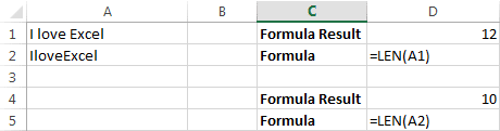
Notice the difference in the formula results: 10 characters without spaces in between the words, 12 with spaces between the words.
5. TRIM
Formula: =TRIM(A1)
Gets rid of any space in a cell, except for single spaces between words. I’ve found this formula to be extremely useful because I’ve often run into situations where you pull data from a database and for some reason extra spaces are put in behind or in front of legitimate data. This can wreak havoc if you are trying to compare using IF statements or VLOOKUP’s.
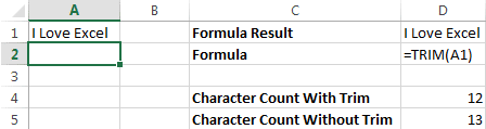
I added in an extra space behind “I Love Excel”. The TRIM formula removes that extra space. Check out the character count difference with and without the TRIM formula.
6. RIGHT, LEFT, MID
Formulas: = RIGHT(text, number of characters), =LEFT(text, number of characters), =MID(text, start number, number of characters).
(Note: In all of these formulas, wherever it says “text” you can use a cell reference as well)
These formulas return the specified number of characters from a text string. RIGHT gives you the number of characters from the right of the text string, LEFT gives you the number of characters from the left, and MID gives you the specified number of characters from the middle of the word. You tell the MID formula where to start with the start_number and then it grabs the specified number of characters to the right of the start_number.

I used the LEFT formula to get the first word. I had it look in cell A1 and grab only the 1st character from the left. This gave us the word “I” from “I love Excel”
I used the MID formula to get the middle word. I had it look in cell A1, start at character 3, and grab 5 characters after that. This gives us just the word “love” from “I love Excel”
I used the RIGHT formula to get the last word. I had it look at cell A1 and grab the first 6 characters from the right. This gives us “Excel” from “I love Excel”
7. VLOOKUP
Formula: =VLOOKUP(lookup_value, table_array, col_index_num, range_lookup)
By far my most used formula. The official description of what it does: “Looks for a value in the leftmost column of a table, and then returns a value in the same row from a column you specify…”. (See the full explanation of VLOOKUP) Basically, you define a value (the lookup_value) for the formula to look for. It looks for this value in the leftmost column of a table (the table_array).
Note: If at all possible use a number for the lookup_value. This makes it a lot easier to make sure the data you are getting back is a correct match.
If it finds a match of the “lookup_value” in the left column of the “table_array” it will return the value in the column you specify using the “index_num”. The “index_num” is relative to the left mostcolumn. So, if you have the table_index look in column A and you want what is returned to be what’s in column B the “index_num” would be 2 because the leftmost column, column A in this case, is the 1st column in the table array and column B is the 2nd column (hence the 2 for the index number). If you want what is in column C to be returned you’d put 3 for the index_num. The “range_lookup” is a TRUE or FALSE value. If you put TRUE it will give you the closest match. If you put FALSE it will only give you an exact match. I only use FALSE when using the VLOOKUP formula.
Example:
You have 2 lists: 1 with a sales person’s ID and the sales revenue for the quarter. Another with the sales person’s ID and the sales person’s name. You want to match up the sales person’s name to the sales person’s revenue numbers for the quarter. They are all jumbled around so to manually match this, even for a small number of salesmen would leave room for a high margin of error and take a lot of time.
The first list goes from A1 to B13. The 2nd list goes from D1 to E25.
In cell C1 I would put the formula =VLOOKUP(B18, $A$1:$B$13, 2, FALSE)
B18 = the lookup_value (the sales person’s ID. This is a number that appears on both lists.)
$A$1:$B$13 = the “table_array”. This is the area I want the formula to search the leftmost column (column E in this case) for the “lookup_value”. I went to F because if it finds match in column E, I want it to return what’s in column F. (The money signs are there so that the table_array will stay the same no matter where the formula is moved or copied to. This is called an absolute reference.)
2 = the index_num. This tells the formula the number of columns away from the left most column to return in case of match. So, if you find a match between the lookup_value and the leftmost column of the table array, return what’s in the same row in the 2nd column of the table (the 1st column is always the leftmost column. It starts at 1, not 0).
FALSE= tells the formula I want it to only return the value if it’s an exact match.
I would then copy and paste that formula along all the cells in column C next to the first list. This would give me a perfectly aligned list with the sales person’s ID, sales person’s revenue for the quarter, and the sales person’s name.

In order to get a nice neat list of Sales Person ID, Sales Person Name, and Sales Person Revenue all next to each other I used the VLOOKUP formula to compare 1 list to another.
This is a complicated formula, but an extremely useful one. Check out some other examples: Vlookup Example,Microsoft’s Official Example.
**Learn more about the VLOOKUP function in this on-demand, online course. FREE preview**
8. IF Statements
Formula: =IF(logical_statement, return this if logical statement is true, returnthis if logical statement is false)
When you’re doing an analysis of a lot of data in Excel there are a lot of scenarios you could be trying to discover and the data has to react differently based on a different situation.
Continuing with the sales example: Let’s say a salesperson has a quota to meet. You used VLOOKUP to put the revenue next to the name. Now you can use an IF statement that says: “IF the salesperson met their quota, say “Met quota”, if not say “Did not meet quota” (Tip: saying it in a statement like this can make it a lot easier to create the formula, especially when you get to more complicated things like Nested IF Statements in Excel).
It would look like this:
In the example with the VLOOKUP we had the revenue in column B and the person’s name in column C (brought in with the VLOOKUP). We could put their quota in column D and then we’d put the following formula in cell E1:
=IF(C3>D3, “Met Quota”, “Did Not Meet Quota”)
This IF statement will tell us if the first salesperson met their quota or not. We would then copy and paste this formula along all the entries in the list. It would change for each sales person.

Having the result right there from the IF statement is a lot easier than manually figuring this out.
9. SUMIF, COUNTIF, AVERAGEIF
Formulas: =SUMIF(range, criteria, sum_range), =COUNTIF(range, criteria), =AVERAGEIF(range, criteria, average_range)
These formulas all do their respective functions (SUM, COUNT, AVERAGE) IF the criteria are met. There are also the formulas: SUMIFS, COUNTIFS, AVERAGEIFS where they will do their respective functions based on multiple criteria you give the formula.

I use these formulas in our example to see the average revenue (AVERAGEIF) if a person met their quota, Total revenue (SUMIF) for the just the sales people who met their quota, and the count of sales people who met their quota (COUNTIF)
10. CONCATENATE
A fancy word for combining data in 2 (or more) different cells into one cell. This can be done with the Concatenate excel formula or it can be done by simply putting the & symbol in between the two cells. If I have “Steve” in cell A1 and “Quatrani” in cell B1 I could put this formula: =A1&” “&B1 and it would give me “Steve Quatrani”. (The “ “ puts aspace in between what you are combining with the &). I can use =concatenate(A1, “ “, B1) and it will give me the same thing: “Steve Quatrani”

Finding The Right Excel Formulas For The Job
There are 316 built in functions in Excel. You’re not going to sit there and memorize what all of them do (or at least I hope not!). Luckily Excel has a built in wizard that helps you find the correct formula for what you’re looking to do (if there is one).
Click the “fx” next to the formula bar in Excel

This brings up a menu and in there you can type in a description of what you are trying to do and it will bring up the correct excel formula:

I typed in “remove extra spaces” and it returned the TRIM formula that we went over earlier.
No comments:
Post a Comment